Palos Verdes Homes & South Bay Real Estate
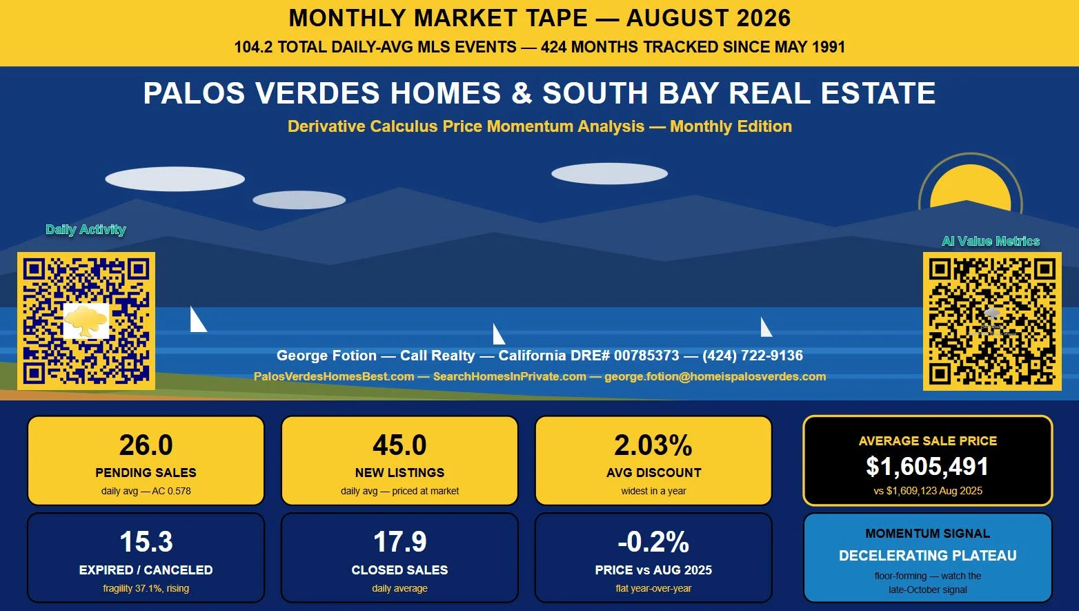
45.0 New Listings per day avg | 26.0 Pending Sales per day avg | 17.9 Closed Sales per day avg | 15.3 Expired & Canceled per day avg | $1,605,491 Avg Sale Price −0.2% vs Aug 2025 | 2.03% Avg Discount list-to-sale spread | 104.2 Total Events daily avg, all categories |
Executive Summary — What 424 Months of Tape Say About Right Now
August closed the summer with a market that is balanced on the surface and quietly softening underneath. The headline: the average South Bay/Palos Verdes sale price came in at $1,605,491 — within $4,000 (−0.2%) of August 2025. Prices have gone flat, not down. But the first and second derivatives of this market — the metrics I track every single day — are telling a richer story.
The monthly Absorption Coefficient (pendings ÷ new listings) printed 0.578: for every 1,000 homes that came to market in August, 578 went under contract. That sits at the 39th percentile of all 424 months and below the 10-year average of 0.742 — demand is real but no longer outrunning supply. Meanwhile the monthly Escrow Fragility reading — failed listings as a share of all monthly exits — hit 37.1%, its fifth consecutive monthly increase and its highest level since January. More than one in three listings leaving the market right now is leaving without a buyer.
Here is the tension every client should understand: sellers as a group have already adjusted — the average new listing in August was priced at $1,593,712, essentially the same as the average sale price. Correctly priced homes are transacting near ask. But the average closed discount widened to 2.03%, the largest negotiating spread in roughly a year, and the smoothed year-over-year price line has now been negative for seven straight months. Historically, that exact signature — flat-to-slightly-negative YoY, mediocre absorption, rising fragility — is what a floor being formed looks like, not a crash. The full statistical case is in the year-over-year section below.
0.578 MONTHLY AC — AUG 2026 39th pctile of 424 months | 37.08% MONTHLY EFI — AUG 2026 5th straight monthly rise | AC 20.000 DAILY SERIES — SESSION 99 (AUG 31) all-time record; EFI 16.67% | AC 1.607 DAILY CUMULATIVE S1–99 EFI 21.67% — anchor values |
Monthly Metrics Table — August 2026
| Metric | August 2026 | What It Means |
|---|---|---|
| New Listings (daily avg) | 45.0 | Down from 49.9 in July — supply is tightening into fall |
| Pending Sales (daily avg) | 26.0 | AC = 0.578: 578 homes going under contract per 1,000 new listings |
| Closed Sales (daily avg) | 17.9 | Steady vs 18.1 in July; pipeline of 26 pendings supports fall closings |
| Expired & Canceled (daily avg) | 15.3 | 37.1% of monthly exits are failed listings — 5th consecutive monthly rise in the fragility reading |
| Average Sale Price | $1,605,491 | Essentially flat year-over-year (−$3,632, −0.2%) |
| Average List Price, New Listings | $1,593,712 | New inventory is being priced AT market — sellers have adjusted |
| Average Discount (list vs sale) | 2.03% | Widest since last fall; buyers are recovering negotiating room |
| Success Ratio (CS+PS)/XK | 2.87 | 2.87 successes per failure — solid, but off the 3.3–3.4 spring pace |
Year-Over-Year Analysis — Do the YoY Columns Predict Future Prices?
Your monthly tape carries two columns most agents never compute: “Month vs Previous Year’s Same Month” (the dollar change vs the same month last year) and “% Change from Same Month Last Year”. I ran the full 400+ month history through a forward-return test: does this year-over-year reading actually correlate with where prices go next?
Finding 1 — YoY is a momentum gauge, not a contrarian signal. The raw YoY% reading correlates +0.33 with price change over the following 12 months. Sorted into quintiles, months in the strongest YoY quintile (~+15%) were followed by an average +11.6% over the next year; months in the weakest quintile (~−10%) were followed by −1.1%. Appreciation persists; deep declines tend to stall rather than compound.
Finding 2 — where we are now. August’s YoY print is −0.2%, and the 12-month smoothed YoY sits at −4.9%, negative for seven consecutive months — the 11th percentile of history. That lands us in the weak quintile. But here is the critical base rate: across the 62 prior months in which smoothed YoY had been negative for six months or longer, the average price change over the following 12 months was +0.1%, with 53% of outcomes positive. Translation: this signature marks the flat part of the cycle — the floor — far more often than it marks the edge of a cliff.
Finding 3 — the derivatives lead better than YoY itself. The 12-month Absorption Coefficient correlates +0.69 with price change two years out, and the fragility reading correlates −0.62. Top-quintile absorption months were followed by +13.7% average 12-month gains; top-quintile fragility months by −4.7%. Today’s combination — AC at the 36th percentile, fragility at the 57th — projects a flat-to-low-single-digit 12-month path, with the upside trigger being AC recovering above ~0.68 (its historical third quintile) and the fragility streak breaking. My separate 1,837-week WEEKTICK model projects exactly that convergence arriving late October–November 2026, with +4–8% appreciation by mid-2027 if it confirms.
Advice for Sellers
- Price at the market, not above it — the tape proves your neighbors already have. August’s new listings averaged $1,593,712 against an average sale of $1,605,491. The sellers succeeding right now are priced within 2–3% of closed comparables from day one. With 37% of monthly exits now ending in expiration or cancellation, an aspirational price is the single biggest predictor of joining the failure pile.
- Your competition is thinning — use it. New listings fell from 49.9/day in July to 45.0/day in August, and fall traditionally cuts supply further. A sharp launch in September–October faces the least competition since spring, while 26 buyers a day are still writing accepted offers.
- Fortify the escrow, because escrows are where deals now die. With the fragility reading at 37.1% and rising five straight months, do the pre-listing inspection, pre-empt the appraisal conversation with a comp package, and vet buyer financing hard before accepting. The closed-to-pending ratio of 0.69 says roughly three in ten contracts are not converting on schedule.
- If you’re planning to sell into 2027, watch my October signal. The weekly model’s demand indicator is projected to cross its strong-market threshold late October–November. If it confirms, spring 2027 likely brings better pricing — but also more competition. I’ll tell my database the week it happens; make sure you’re on the list.
Advice for Buyers
- This is the low-FOMO window the tape rarely gives you. Prices are flat year-over-year, the average discount has widened to 2.03% — the most negotiating room in about a year — and the historical base rate after seven negative smoothed-YoY months is a flat forward year. You can be selective without racing appreciation.
- Hunt the failure pool. 15.3 listings a day expired or canceled in August. These owners already told the market their price was wrong; many still need to sell. A re-approach 30–60 days later, with data, is where the genuine below-market deals in this market live.
- Move before the convergence, not after it. Absorption at the 36th percentile with fragility elevated is precisely the setup that historically precedes recovery — top-quintile absorption regimes delivered +13.7% forward years. If my late-October threshold signal confirms, the leverage you hold today shrinks. The strategic play is a fall 2026 purchase ahead of a projected 2027 upturn.
- Underwrite the escrow like a seller would. In a 37% fragility market, listing agents are prioritizing certainty over the last dollar. Tight contingency windows, verified funds, and a clean lender letter routinely beat a slightly higher but shakier offer — that is a price discount you buy with preparation, not cash.
Strategic Opportunities — Four Plays for Fall 2026
- The Expired Re-Entry Play (buyers & investors): systematically track August–September expirations; approach with closed-comp evidence and a clean offer. The 2.87 success-per-failure ratio means the failures are concentrated among mispriced properties — exactly where negotiated value hides.
- The Supply-Gap Launch (sellers): list into the September–October inventory trough (45.0 new/day and falling) rather than waiting for spring 2027, when the projected demand recovery will also bring back your competition.
- The Flat-Market Trade-Up (move-up owners): when the whole market is flat, the spread between your sale and your purchase is at its cheapest. A $1.6M-to-$2.4M trade costs the same relative gap it will after a broad +5% year — except the bigger home’s 5% is a bigger number. Flat markets subsidize trade-ups.
- The Convergence Front-Run (everyone): two independent models — this monthly tape’s derivative structure and the 1,837-week WEEKTICK series — point to the same late-October–November 2026 inflection window. Position before confirmation; react-to-headlines pricing arrives months later.
First derivative (velocity): Monthly AC = 26.0 pendings ÷ 45.0 new listings = 0.578 — 39th percentile of 424 months, below the 10-year mean of 0.742. Demand velocity is positive but sub-trend. On the daily tape, today’s Session 99 printed an all-time record AC of 20.000 on a supply-collapse single new listing — the daily and monthly lenses agree on the cause: supply is contracting faster than demand.
Second derivative (durability): the monthly fragility reading — expired & canceled as a share of all exits — is 37.1%, rising five consecutive months. Acceleration is negative: each marginal month is converting listings to closings slightly less efficiently. The daily EFI, by contrast, sits at a healthy 16.67% with a cumulative series anchor of 21.67% — short-run escrows are holding; it’s the stale-listing pool doing the failing.
The calculus conclusion: price level flat (f), velocity positive-but-subpar (f′), acceleration mildly negative (f′′) — a decelerating plateau. Historical analogs resolve upward when AC clears ~0.68 and the fragility streak breaks. Watch October.
I have tracked this market every single day for over 45 years. I can run this exact derivative analysis on your specific property, your neighborhood, or the home type you want to own next.
(424) 722-9136 • george.fotion@homeispalosverdes.com
PalosVerdesHomesBest.com • SearchHomesInPrivate.com • calendly.com/george-fotion
Don’t miss the charts at the end of this post!
Click image above; navigate to the DAILY TRENDS
Want to know more about the Department of Justice Settlement with the National Association of Realtors? You need to understand this because Buyers and Brokers must comply. Read more about it here
Click here for WEEKLY trends
George Fotion • Call Realty • DRE# 00785373 • (424) 722-9136
| Column | Aug 2026 (3-mo MA) | Aug 2028 Projection | 24-Mo Δ | Guardrail |
|---|---|---|---|---|
| New Listings (daily avg) | 48.4 | 58.4 | +20.6% | capped at historical extreme |
| Average List Price — New Listings | $1,613,179 | $1,673,745 | +3.8% | capped at historical extreme |
| Expired & Canceled (daily avg) | 15.0 | 17.0 | +13.3% | within rails |
| Average List Price — Expired & Canceled | $1,603,864 | $1,663,487 | +3.7% | capped at historical extreme |
| Pending Sales (daily avg) | 27.5 | 30.1 | +9.2% | capped at historical extreme |
| Average List Price — Pending Sales | $1,597,529 | $1,751,327 | +9.6% | capped at historical extreme |
| Closed Sales (daily avg) | 17.3 | 19.2 | +11.1% | within rails |
| Average Sale Price — Closed Sales | $1,561,098 | $1,714,683 | +9.8% | within rails |
| Average % Discount (List vs Sale) | 1.13% | 1.16% | +2.2% | capped at historical extreme |
| Absorption Coefficient #PS / #NL | 0.569 | 0.454 | -20.2% | capped at historical extreme |
| Conversion Ratio #CS / #PS | 0.628 | 0.635 | +1.0% | capped at historical extreme |
| Success-per-Failure Ratio (#CS+#PS) / #XK | 2.979 | 2.804 | -5.9% | within rails |
| Supply / Demand Balance | -20.9 | -28.3 | -35.6% | within rails |
Model per column: 3-month moving average → recent slope (OLS, last 36 months) converging exponentially toward the long-run slope (OLS, last 120 months) → month-of-year seasonal factors from the last 10 years → guardrails clipping the path to each column’s own historical extreme 24-month moves. Columns flagged “capped at historical extreme” had raw extrapolations exceeding anything the series has done in 424 months — the rail, not the raw trend, governs.
The one divergence to respect: each column is projected independently, and the mechanics disagree in one place — the sale-price MA projects +9.8% by Aug 2028 (≈+4.8%/yr, consistent with the WEEKTICK model’s +4–8% by mid-2027) while the Absorption Coefficient path drifts down toward 0.45 as projected new listings (+20.6%, rail-capped) outgrow pendings (+9.2%). Both cannot be fully right: sustained sub-0.50 absorption has historically preceded flat, not +5%/yr, pricing. Read the price projection as the upper path, conditional on absorption stabilizing above ~0.55 — which is exactly what the late-October/November convergence signal will confirm or deny. If AC follows its projected path instead, expect the flat-floor scenario from the quintile analysis (≈0 to +2%/yr).
Scale note: the Supply/Demand Balance “−35.6%” is a percentage of a negative level (−20.9 → −28.3 daily deficit) — the meaningful read is a widening supply shortfall of about 7 events/day, well inside historical rails, and structurally supportive of the price floor.


PalosVerdesHomesBest.com • SearchHomesInPrivate.com • calendly.com/george-fotion