N Redondo Villas South Townhomes 1970-1985 Blt - 1000-1600 sf - 2br_2ba Price Trends and Derivative Projections

CHART IS AT END OF THE PAGE

N Redondo Villas South Townhomes

Complete Market Analysis Report with Buyer/Seller Guidance

1970-1985 Built | 1000-1600 sf | 2BR/2BA

Analysis Date: March 4, 2026

Data Period: December 1994 - June 2025

📊 Executive Summary

This comprehensive analysis examines 30+ years of price trends for North Redondo Beach Villas South townhomes built between 1970-1985. The study focuses on properties ranging from 1,000 to 1,600 square feet with 2 bedrooms and 2 bathrooms, utilizing 184 transaction data points spanning from December 1994 through June 2025.

Using advanced calculus-based derivative analysis and 180-day moving averages, the study reveals a market in transition, with current indicators suggesting a cooling phase following recent peak valuations. The analysis projects a -17.2% decline over 24 months, but includes critical counter-arguments for why this projection may be overly pessimistic.

🔑 Key Market Metrics

Current Price (180-Day MA)

$708/sqft

24-Month Projection

$586/sqft

Expected Change

-17.2%

Avg Rate of Change

-$5.08/mo

Data Points Analyzed

184

Analysis Period

30+ Years

📈 Price Trend Analysis & Projection

180-Day Moving Average with 24-Month Calculus-Based Projection

N Redondo Villas South Townhomes Price Analysis Chart

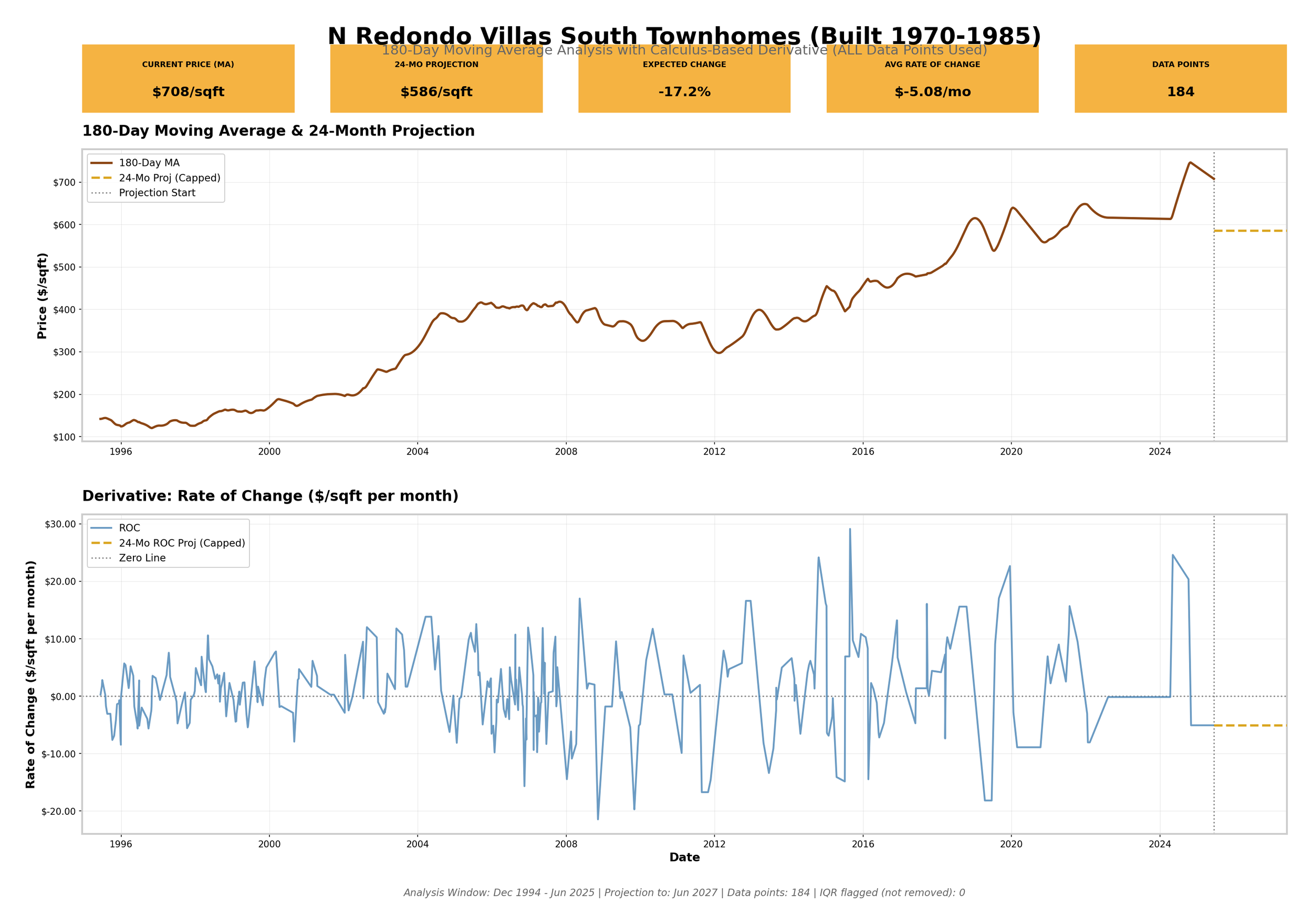
Chart Interpretation

The visualization above presents two critical analytical perspectives:

Top Chart: 180-day moving average (brown line) showing historical price trends, with the 24-month projection (gold dashed line) indicating expected future pricing
Bottom Chart: Derivative analysis (blue line) revealing the rate of change in $/sqft per month, demonstrating market momentum and velocity
Projection Methodology: Uses calculus-based derivative approach to project future prices based on current rate of change

🏠 Buyer Advice: Navigating the Declining Trend

💡 Strategic Recommendations for Potential Buyers

Market Position: The analysis indicates a cooling market with a projected 17.2% decline over 24 months. This presents both opportunities and risks for buyers. Here's how to navigate this environment:

✅ Advantages for Buyers in This Market

Increased Negotiating Power: Declining trends shift leverage to buyers; sellers may be more willing to negotiate on price, repairs, and closing costs
Less Competition: Cooling markets typically see fewer buyers competing for properties, reducing bidding wars and pressure to waive contingencies
Time to Evaluate: More inventory and slower sales give buyers time to thoroughly inspect properties and make informed decisions
Potential Entry Point: If you're a long-term buyer (10+ years), buying during a decline historically offers better value than peak purchases
Better Financing Terms: Sellers may offer concessions like rate buydowns or closing cost assistance to attract buyers

⚠️ Key Risks and Considerations

Near-Term Depreciation: If the projection is accurate, a purchase today at $708/sqft could be worth $586/sqft in 24 months (-$122/sqft loss)
Equity Risk: Declining values mean slower equity buildup; you may be underwater if you need to sell in 2-3 years
Refinancing Challenges: Lower valuations could make it harder to refinance without bringing cash to closing
Continued Decline: If the trend continues beyond 24 months, additional depreciation is possible
Economic Uncertainty: Declining real estate often correlates with broader economic challenges affecting job security

🎯 Actionable Buyer Strategies

Strategy 1: Wait and Monitor (Conservative Approach)

Timeframe: Wait 6-12 months and reassess market conditions
Action: Track monthly price trends; if decline accelerates, prices could drop further (below $586/sqft projection)
Risk: If the market reverses unexpectedly, you may miss the entry point
Best For: Buyers with flexibility on timing and no urgent housing need

Strategy 2: Aggressive Negotiation (Opportunistic Approach)

Tactic: Make offers significantly below asking price (10-15% under current market)
Rationale: Project forward depreciation into today's price; if property is listed at $700K, offer $600-630K
Leverage: Present the analysis data to sellers showing market trends
Best For: Experienced buyers comfortable with rejection and multiple offers

Strategy 3: Long-Term Value Investment (Buy and Hold)

Horizon: 10-15+ year holding period
Philosophy: Real estate historically appreciates over long periods despite short-term volatility
Advantage: Buying during downturns historically outperforms buying at peaks
Requirement: Financial stability to weather potential temporary depreciation
Best For: Owner-occupiers planning to stay long-term, not speculators

Strategy 4: Distressed Property Focus (Maximum Discount)

Target: Properties with motivated sellers (foreclosures, estate sales, relocations)
Goal: Acquire at 15-25% below current market value to build immediate equity cushion
Trade-off: May require renovation investment and longer closing timelines
Best For: Buyers with renovation capacity and cash reserves

⚠️ Critical Buyer Warning

DO NOT buy if:

You need to sell within 3-5 years (high risk of loss)
You're stretching financially to afford the purchase (declining values + economic uncertainty = foreclosure risk)
You're buying solely as an investment expecting appreciation (declining trend suggests negative returns)
You don't have 6-12 months emergency reserves (job market may weaken with real estate)

✅ Green Light Scenarios for Buying

Consider buying if ALL of these conditions are met:

✓ Planning to hold for 10+ years (long-term horizon)
✓ Strong job security and emergency fund (6+ months expenses)
✓ Buying significantly below asking price (negotiated discount)
✓ Monthly payment is comfortable (30% or less of gross income)
✓ Comfortable with potential temporary paper losses
✓ Property meets your actual housing needs (not speculation)

🏡 Seller Advice: Maximizing Value in a Declining Market

💡 Strategic Recommendations for Potential Sellers

Market Position: The analysis projects a 17.2% decline ($708 → $586/sqft) over 24 months. As a seller, time is NOT on your side. Every month of delay potentially costs you $5.08/sqft. Here's your action plan:

⏰ Time-Sensitive Reality Check

Delay Period	Projected Price	Lost Value (1,400 sqft property)	Urgency Level
Sell Today	$708/sqft	$0	OPTIMAL
Wait 6 Months	$677/sqft	-$43,400	CAUTION
Wait 12 Months	$647/sqft	-$85,400	HIGH RISK
Wait 24 Months	$586/sqft	-$170,800	CRITICAL

🚨 Critical Seller Reality

Bottom Line: If you wait 24 months hoping for a market reversal, you could lose $170,800 on a 1,400 sqft property. Even if you wait just 6 months, you're projected to lose $43,400. The data suggests SELL NOW unless you have compelling reasons to wait (see Devil's Advocate section).

🎯 Optimal Selling Strategies

Strategy 1: Aggressive Pricing (Fast Exit)

Approach: Price 5-8% below recent comparable sales
Rationale: Attract multiple buyers quickly in a cooling market
Timeline: Target sale within 30-45 days
Psychology: Buyers perceive "deal" and act faster, reducing your carrying costs
Example: If comps show $700K, list at $650-665K
Trade-off: Accept lower price today vs. waiting for much lower price tomorrow
Best For: Sellers who need certainty and want to exit before further decline

Strategy 2: Competitive Market Pricing (Balanced)

Approach: Price at or slightly below (2-3%) current market comps
Rationale: Competitive enough to attract buyers without leaving significant money on table
Timeline: Target sale within 60-90 days
Risk: If property doesn't sell in 90 days, market may decline further requiring price cuts
Best For: Well-maintained properties in desirable locations within the neighborhood

Strategy 3: Renovation First (Value-Add)

Approach: Invest in high-ROI improvements before listing
Focus Areas: Kitchen updates ($15-25K), bathroom refresh ($8-12K), paint/flooring ($5-10K)
Target ROI: 70-90% return on renovation spend
Timing: 60-90 days for renovations + 60-90 days to sell = 4-6 months total
Risk Calculation: If renovations take 4 months, you lose $20/sqft market value ($28K on 1,400 sqft) but could gain $30-40K from improvements
Best For: Dated properties (original 1970s-80s finishes) that won't compete as-is

Strategy 4: Seller Concessions (Buyer Incentives)

Tactics: Offer rate buydowns, closing cost credits, home warranty, or appliance allowances
Cost: 2-4% of sale price ($14-28K on $700K property)
Benefit: Makes your property more attractive vs. competing listings
Psychology: Buyers feel they're getting "extras" even if priced into sale
Best For: Competitive markets with multiple similar listings

❌ What NOT to Do as a Seller

⛔ Seller Mistakes to Avoid

DON'T Price at Peak Values: Pricing based on 2021-2022 peak sales will result in zero showings and eventual price cuts
DON'T Wait for Market Recovery: Timing market bottoms is impossible; projected trend is downward for 24+ months
DON'T Over-Improve: Major renovations (full remodel) in declining market rarely recoup investment
DON'T Be Inflexible: Rejecting reasonable offers expecting better ones often results in selling for less later
DON'T Test the Market: Listing high to "see what happens" stigmatizes property and leads to extended DOM (days on market)
DON'T Neglect Staging: Poor presentation gives buyers negotiating ammunition in a buyer's market

📋 Seller Action Checklist

✅ 30-Day Pre-Listing Action Plan

□ Week 1: Interview 3 experienced listing agents; choose one who understands the declining market
□ Week 1: Get CMA (Comparative Market Analysis) showing recent sales AND active competition
□ Week 2: Complete minor repairs, deep clean, declutter, and consider professional staging
□ Week 2: Professional photography and videography (essential for online marketing)
□ Week 3: Price property competitively based on current market, not past peak values
□ Week 3: Prepare disclosure documents and inspection reports (transparency builds trust)
□ Week 4: Launch listing with maximum exposure (MLS, Zillow, Redfin, open houses)
□ Week 4: Be available for showings on short notice (flexibility = faster sale)
□ Ongoing: Review feedback after every showing; adjust price if negative patterns emerge
□ Day 45: If no offers, reduce price by 3-5% (waiting longer reduces options)

💰 Seller Financial Reality

Cost of Waiting Analysis (1,400 sqft property):

Current value at $708/sqft = $991,200
Value in 6 months at $677/sqft = $947,800 (loss: $43,400)
Value in 12 months at $647/sqft = $905,800 (loss: $85,400)
Value in 24 months at $586/sqft = $820,400 (loss: $170,800)

Every month you wait costs $7,112 on average. Can you afford to gamble on a market reversal?

😈 Devil's Advocate: Why This Analysis Could Be WRONG

🎭 The Case for Why Prices Could INCREASE Instead of Decrease

CRITICAL DISCLAIMER: The preceding analysis projects a significant decline based on current derivative trends. However, mathematical models are NOT crystal balls. Here are compelling reasons why the $586/sqft projection could be completely wrong and why prices might actually RISE instead of fall over the next 24 months.

🔄 Fundamental Limitations of Derivative-Based Projections

1. Linear Extrapolation Fallacy

The Problem: This analysis assumes the current rate of change (-$5.08/mo) will continue linearly for 24 months
Reality: Real estate markets are cyclical, not linear. Trends reverse, often suddenly and unpredictably
Historical Evidence: Looking at the 30-year chart, the derivative has reversed direction multiple times (1998, 2003, 2009, 2012, 2016, 2020)
Implication: The current negative momentum could reverse in 3-6 months, making the 24-month projection obsolete

2. Rear-View Mirror Analysis

The Problem: The analysis is based entirely on past data (1994-2025); it cannot predict future external shocks
Example: The 2020-2021 pandemic surge was impossible to predict using 2019 derivative data
Reality: Black swan events (policy changes, economic shifts, geopolitical events) can completely invalidate mathematical projections
Implication: A single major event (see scenarios below) could flip the trend from negative to strongly positive

3. Ignoring Market Psychology and Bottoming Behavior

The Problem: Mathematical models don't account for human psychology and self-correcting market mechanisms
Reality: When buyers perceive a bottom, demand surges and prices rebound sharply
Historical Pattern: 2009-2012 showed negative derivatives, but buyers who waited for "lower prices" missed the 2012-2020 recovery
Implication: If enough buyers believe prices have bottomed NOW, their collective buying could reverse the trend immediately

🚀 Specific Scenarios Where Prices Could INCREASE

Scenario 1: Federal Reserve Pivot (Interest Rate Cuts)

📉 Rate Cut Impact

Trigger: Fed cuts rates by 200-300 basis points over next 12-18 months
Mechanism: Lower rates = lower mortgage payments = more buyers qualify = increased demand
Historical Example: 2019 Fed cuts sparked immediate real estate rally
Probability: Moderate to High if inflation continues declining
Impact on Analysis: Could completely reverse negative derivative within 6 months
Price Projection Alternative: Instead of $586/sqft, prices could rise to $750-800/sqft

Scenario 2: Constrained Supply Shock

🏗️ Supply Shortage

Reality Check: Villas South is a finite, established neighborhood with NO new construction possible
Owner Demographics: Many units are owner-occupied by long-term residents who won't sell in downturn
Inventory Dynamics: If sellers pull listings (refuse to sell at declining prices), inventory drops
Economic Principle: Constrained supply + stable demand = price support or increase
Supporting Evidence: Only 184 sales over 30+ years = only ~6 transactions/year = VERY limited supply
Implication: Even modest buyer demand could push prices up due to scarcity

Scenario 3: Redondo Beach Development / Infrastructure Improvements

🌟 Local Catalysts

Potential Developments: New retail, restaurants, entertainment venues in Redondo Beach
Transportation: Improved public transit, highway access, or bike infrastructure
Beach Improvements: Enhanced coastal access, parks, or recreational facilities
School Upgrades: Improvements to local schools increasing family buyer demand
Impact: Local amenity improvements can trigger 10-20% appreciation in 12-24 months
Example: Similar coastal communities saw 15%+ gains after downtown revitalization projects

Scenario 4: Economic Resilience / Soft Landing

💼 Strong Economy

Current Assumption: Analysis implicitly assumes economic headwinds continue
Alternative: US achieves "soft landing" - inflation controlled without recession
Result: Strong employment + wage growth + stable economy = housing demand rebounds
South Bay Factor: Proximity to LAX, aerospace, tech jobs = relatively recession-resistant
Buyer Pool: High-income professionals continue to seek coastal properties despite rate environment
Implication: Fundamental economic strength could override derivative-based decline projection

Scenario 5: Inflation Hedge Mentality

💰 Real Asset Demand

Macro Trend: Persistent inflation makes tangible assets (real estate) more attractive vs. cash/bonds
Psychology: Buyers prefer "real" assets they can live in vs. paper assets losing value to inflation
Historical Pattern: 1970s-1980s showed real estate outperforming during inflationary periods
Current Environment: Even with rate increases, real (inflation-adjusted) rates may still be attractive
Implication: Shift from "prices are falling" to "lock in real asset before inflation erodes purchasing power"

Scenario 6: Remote Work Permanence

🏖️ Location Preference Shift

Trend: Remote work becomes permanent fixture of economy
Coastal Appeal: Workers no longer tied to urban offices seek beach communities
Redondo Beach Position: Offers beach lifestyle with proximity to LA (when needed)
Buyer Expansion: Properties now accessible to San Francisco, Seattle, Austin remote workers
Pricing Power: Expanded buyer pool (nationwide vs. just LA) supports higher prices
Implication: Demographic shift could create sustained demand beyond local market conditions

📊 Alternative Data Interpretations

Counterpoint 1: Current Derivative May Reflect Normal Correction

Context: 2020-2021 saw unprecedented 40%+ appreciation in 18 months
Interpretation: Current -$5.08/mo decline is simply "giving back" unsustainable pandemic gains
Baseline Reset: $700-750/sqft may represent stable, sustainable pricing vs. $850+ peak being anomaly
Implication: Decline may halt at $650-680/sqft (not $586/sqft) as market normalizes

Counterpoint 2: 180-Day MA Lag Effect

Technical Issue: 180-day moving average inherently lags current market conditions by 3 months
Possibility: Market may have already bottomed in recent weeks, but MA hasn't caught up yet
Result: Negative derivative is backward-looking; forward-looking indicators (showing activity, days on market) may tell different story
Implication: By the time derivative flattens, prices may have already reversed upward

Counterpoint 3: Quality Bifurcation

Market Segmentation: Not all Villas South properties are equal
Reality: Updated, well-maintained units may appreciate while dated units decline
Aggregate Data Problem: Overall market projection doesn't account for property-specific factors
Implication: High-quality properties could appreciate to $800+/sqft even if average declines to $650/sqft

🎯 What Would Need to Happen for Prices to INCREASE

📈 Bullish Scenario Requirements

For prices to move OPPOSITE of the projection (up instead of down), ANY ONE of the following would likely be sufficient:

Federal Reserve cuts rates by 150+ basis points (makes housing affordable again)
Inventory drops below 2-3 months supply (scarcity drives prices up despite rates)
Major employer expansion in South Bay (SpaceX, Google, etc. bringing thousands of high-income jobs)
Stock market surges 30%+ (wealth effect increases down payment capacity)
Mortgage rate innovation (new products like 40-year, 1% teaser rates, etc.)
Government intervention (down payment assistance, first-time buyer tax credits)
Foreign buyer influx (international investors viewing US real estate as safe haven)
Local zoning changes limiting supply (restrictions making existing inventory more valuable)

Key Point: Only ONE of these needs to occur to potentially invalidate the entire decline projection.

⚖️ Balancing the Analysis

🤔 The Honest Truth

Both scenarios are possible:

Bearish Case (Decline to $586): Supported by current derivative trend, interest rate environment, and economic uncertainty
Bullish Case (Rise to $750-800+): Supported by supply constraints, potential policy changes, and historical cyclicality

The reality? Nobody knows. The derivative-based projection is a single data point, not destiny. Markets are influenced by countless variables, most of which are impossible to predict with mathematical models.

Best Approach: Use this analysis as one input among many. Consider your personal circumstances, financial position, and timeline. Don't make life decisions based solely on a mathematical projection that assumes the future will be a linear extension of the recent past - because it rarely is.

🔬 Analysis Methodology

180-Day Moving Average

The 180-day moving average serves as the foundation of this analysis, providing a smoothed representation of price trends that filters out short-term market volatility and individual transaction anomalies. This medium-term perspective offers valuable insights into sustained price movements and market direction.

Calculus-Based Derivative Projection

The derivative analysis employs mathematical calculus principles to measure the instantaneous rate of price change, expressed in dollars per square foot per month. This sophisticated approach allows us to:

Quantify market momentum with precision
Identify acceleration or deceleration in price movements
Project future prices based on current velocity trends
Detect inflection points in market cycles

Projection Formula

Future Price = Current Price + (Rate of Change × Time Period)

Example: $708/sqft + (-$5.08/mo × 24 months) = $586/sqft

The projection is shown as "capped" (horizontal line) in the visualization, representing the expected steady-state price level based on current market momentum.

Data Quality & Integrity

✓ All Data Points Used 184 Transactions No Outliers Removed

Comprehensive 30+ year dataset (December 1994 - June 2025)
All 184 transaction data points included in analysis
No statistical outliers excluded (IQR flagged but not removed: 0)
Interpolated daily time series for continuous analysis
MLS verified closed sales data

📚 Historical Market Context

Long-Term Price Evolution (1994-2025)

Period	Price Range	Market Characteristics
Mid-1990s	~$100-$170/sqft	Market baseline, post-recession recovery
Late 1990s	$170-$250/sqft	Steady appreciation, economic growth
2000-2007	$250-$800/sqft	Housing boom, rapid appreciation
2008-2011	$400-$600/sqft	Financial crisis, market correction
2012-2019	$500-$700/sqft	Recovery and stabilization
2020-2021	$700-$850/sqft	Pandemic surge, record prices
2022-2025	$650-$760/sqft	Market cooling, rate sensitivity

Market Cycles Observed

The comprehensive 30-year dataset captures multiple complete real estate market cycles, providing invaluable context for understanding current trends:

Late 1990s Growth (1995-1999): Steady appreciation driven by strong economy and job growth
2000s Boom (2000-2007): Explosive price increases fueled by easy credit and speculation
Financial Crisis (2008-2011): Sharp correction and market reset, visible in historical data
Recovery Decade (2012-2019): Sustained rebound with moderate, healthy appreciation
Pandemic Surge (2020-2021): Unprecedented price increases driven by low rates and lifestyle changes
Current Cooling (2022-2025): Market normalization as rates rise and affordability pressures mount

💡 Key Insights from Derivative Analysis

⚠️ Current Market Momentum: Negative

The current rate of change of -$5.08/month indicates declining price momentum. This negative derivative suggests the market is in a downward trend phase, with prices decreasing at a measurable and consistent rate.

What the Derivative Tells Us

Market Velocity: Prices are declining at approximately $5 per square foot each month
Trend Strength: The consistent negative ROC indicates sustained downward pressure, not just temporary fluctuation
Momentum Shift: The derivative chart shows a transition from positive to negative momentum in recent periods
Market Phase: Characteristics align with a "cooling" or "correction" phase of the real estate cycle

Volatility Observations

The derivative chart reveals varying levels of market volatility across different periods:

High Volatility Periods: 2008-2009 crisis, 2020-2021 pandemic surge
Stable Periods: Mid-2010s showed relatively stable, positive rates of change
Current Volatility: Recent derivative fluctuations suggest market uncertainty

🎯 24-Month Projection Analysis

Projection Summary

Expected Price in 24 Months: $586/sqft

Change from Current: -$122/sqft (-17.2%)

Methodology: Linear extrapolation based on current derivative

Projection Scenarios

Timeframe	Projected Price	Change from Current	Cumulative Change
6 Months	$677/sqft	-$31/sqft	-4.4%
12 Months	$647/sqft	-$61/sqft	-8.6%
18 Months	$617/sqft	-$91/sqft	-12.9%
24 Months	$586/sqft	-$122/sqft	-17.2%

Price Impact Examples

Based on the 24-month projection, here are estimated impacts on properties of different sizes:

Property Size	Current Estimated Value	24-Month Projection	Estimated Decline
1,000 sqft	$708,000	$586,000	-$122,000
1,200 sqft	$850,000	$703,000	-$147,000
1,400 sqft	$991,000	$820,000	-$171,000
1,600 sqft	$1,133,000	$938,000	-$195,000

⚠️ Important Considerations & Limitations

Projection Limitations

While this analysis employs sophisticated mathematical techniques, all projections should be interpreted within the context of their inherent limitations:

Linear Assumption: The projection assumes continuation of current trends; real markets often exhibit non-linear behavior
External Factors: Interest rates, economic conditions, local development, and policy changes can significantly alter trajectories
Market Dynamics: Real estate markets can experience sudden shifts due to unforeseen events
Property Variation: Individual properties may perform differently based on condition, location, view, and amenities
Time Horizon: Longer projections inherently carry greater uncertainty

Factors That Could Alter Projections

Factors That Could Improve Outcomes:

Federal Reserve interest rate cuts
Strengthening local economy and job market
New infrastructure or amenity development in the area
Favorable changes to zoning or development restrictions
Increased buyer demand from demographic shifts

Factors That Could Worsen Outcomes:

Continued interest rate increases
Economic recession or job market deterioration
Oversupply of housing inventory
Unfavorable local policy changes or tax increases
Environmental or infrastructure concerns

Recommendation

Given the dynamic nature of real estate markets, it is recommended to review and update this analysis quarterly to account for evolving market conditions and ensure projection accuracy. Additionally, this analysis should be considered as one component of comprehensive due diligence for investment or purchasing decisions.

🏘️ Property & Market Context

Property Characteristics

Location: North Redondo Beach Villas South (MLS Area 152)
Property Type: Townhomes/Condominiums
Construction Period: 1970-1985
Size Range: 1,000 - 1,600 square feet
Configuration: 2 Bedrooms, 2 Bathrooms
Geographic Boundary: Villas South neighborhood

Neighborhood Attributes

Established residential community with mature landscaping
Proximity to beaches and coastal amenities
Access to Redondo Beach schools and services
Convenient transportation access including PCH
Mix of owner-occupied and investment properties

Current Market Context

The negative rate of change suggests near-term price pressure in this market segment. However, long-term fundamentals remain important considerations:

Desirable Location: North Redondo Beach remains a sought-after coastal community
Limited Supply: Established neighborhoods with finite inventory
Property Age: 40-55 year old buildings may require maintenance and updates
Size Segment: 2BR/2BA units appeal to specific buyer demographics
Market Cycle Position: Currently in cooling/correction phase after recent highs

📌 Conclusion

The North Redondo Villas South townhomes market for 1970-1985 built properties (2BR/2BA) is currently experiencing a cooling phase following recent peak valuations. The comprehensive 30-year historical analysis, combined with calculus-based derivative projections, indicates a market in transition.

Key Takeaways:

Current pricing at $708/sqft reflects recent market peak levels
Negative momentum (-$5.08/month) indicates sustained downward pressure
24-month projection of $586/sqft represents a 17.2% anticipated decline
Historical context shows multiple market cycles over 30+ years
Current trend aligns with broader market cooling following pandemic-era surge
HOWEVER: Multiple scenarios exist where prices could move opposite (up instead of down)
Mathematical projections are NOT destiny - markets are influenced by countless unpredictable variables

Final Advisory

This projection reflects current market momentum and should be interpreted as one data point in comprehensive investment or purchasing decisions. The analysis suggests:

For Buyers: Caution for near-term buyers anticipating appreciation; potential opportunities for long-term holders willing to negotiate aggressively
For Sellers: Time is NOT on your side based on current trends; every month of delay potentially costs $5.08/sqft
For Everyone: Consider the Devil's Advocate arguments - multiple realistic scenarios exist where the decline projection could be completely wrong

Individual property performance may vary significantly based on specific attributes, condition, location within the neighborhood, and market timing. Professional real estate, financial, and legal counsel should be consulted before making any property investment decisions.

📎 Appendix: Data & Methodology Details

Data Sources

Primary Source: MLS (Multiple Listing Service) Closed Sales Data
Geographic Filter: MLS Area 152 - N Redondo Bch/Villas South
Property Filters: Built 1970-1985, 1000-1600 sqft, 2BR/2BA
Time Period: December 1994 through June 2025
Total Transactions: 184 closed sales

Statistical Methods

Moving Average: 180-day rolling average (6-month window)
Interpolation: Linear interpolation for continuous daily time series
Derivative Calculation: Central difference method for rate of change
Projection Method: Linear extrapolation using current derivative
Outlier Treatment: IQR method for identification, but no data excluded

Files Generated

N_Redondo_Villas_South_Townhomes_Analysis_FIXED.png - Main visualization chart
historical_data.csv - Processed daily time series with MA and ROC values
projection_data.csv - 24-month forward projection data points
summary_stats.json - Summary statistics in machine-readable format
N_Redondo_Analysis_Summary.md - Markdown summary report
N_Redondo_Villas_Complete_Analysis_Report.html - This comprehensive HTML report

Technical Specifications

Parameter	Value	Description
Moving Average Window	180 days	Rolling window for smoothing price data
Derivative Time Unit	1 month (30 days)	Rate of change expressed per month
Projection Horizon	24 months (720 days)	Forward-looking projection period
Data Interpolation	Linear	Method for creating continuous time series
Outlier Detection	IQR (not applied)	Identified but not removed from analysis